

- Review of State Variable Representation of Systems
- Model Control of Single Input – Single Output Systems (SISO)
- Controllability and Observability
- Pole Placement by State Feedback
- Effect of State Feedback on Controllability and Observability
- Controllable and Observable Companion Forms
- Short Answer Questions
- Long Answer Questions
- Classification of Non-linearities
- Phenomenon Exhibited by the Non - Linearity
- Limit Cycles
- Jump Resonance
- Sub - Harmonic Oscillations
- Singular Points
- Phase Plane Analysis
- Construction of Phase Plane Trajectories
- Isocline Method
- Delta Method
- Frequency Entrainment or Synchronization
- Short Answer Questions
- Long Answer Questions
- Formulation of Optimal Control Problems
- Calculus of Variations, Fundamental Concepts- Functional, Variations of Functional
- Fundamental Theorem of Calculus of Variations
- Boundary Conditions
- Constrained Minimization
- Dynamic Programming
- Hamilton Principle of Optimality
- Jacobi Bellman Equation
- Potryagins Minimum Principle
- Short Answer Questions
- Long Answer Questions
Review of State Variable Representation of Systems
Review of State Variable Representation of Systems
Earlier we have studied several methods of analysis and design of feedback systems such as root locus and frequency response methods [Nyquist, Bode, Nicholas chart etc.]. These are called classical or conventional methods.
These methods require physical systems modelled in the form of 'Transfer Function (TF)'. Even though the transfer function method provides a simple and powerful technique for analysis and design, it suffers from some disadvantages or drawbacks.
-
The transfer function is defined under zero initial conditions only.
-
Transfer function model is applicable to only single input single output systems and Linear time-invariant system.
-
This technique does not provide the internal behaviour of the system. i.e it reveals only input is given and the corresponding outputs. There may be systems where the output of a system stable and the internal elements may have a tendency to exceed their specified ratings.
Examples: Electric motors-short circuit of windings, Temperature change in a vehicle engine.
-
For operating a system in a stable mode it is required to feed back the some of the internal dynamics or variables of a system rather than output alone.
-
The classical design methods are essentially trial and error procedures.
Such above methods are not useful in analysing and designing at least moderate complex systems.
In the view of previous disadvantages due to conventional methods; we consider a more general mathematical representation of a system which, along with output, gives information about the state of the system variables at some predetermined points along the flow of signals.
Such considerations have led to the development of the state variable approach.
It is a direct ’time’ domain approach which provides a basis for the advanced control system or modern control theory and system optimization.
This state variable analysis design is applicable to all types of systems such as
-
Linear system - Non-Linear system
-
Time-invariant system -Time-varying system
-
MIMO, SISO, MISO, SIMO systems
-
The state variable representation is applicable to both systems in continuous time and discrete time cases.
-
By using this new technique, the solution can be easily obtained through digital computers.
-
Analysis and design carried out using initial conditions.
-
The knowledge basic rule of vectors and matrix algebra is required for state space calculations.
The mathematical representation of the dynamics of a system utilizes three variables
i. Input-u(t) (or) U(t)
ii. Output - y(t) (or) Y(t)
iii. State variable- x(t) (or) X(t)
Let us consider an example of a mechanical system, as given in Fig.1.
 Fig.1. Mechanical System for State variables
The mathematical equations of above system are
$$ \frac{dx(t)}{dt}=v(t)$$ ......................................(2)
$$ v(t)=\frac{1}{M}\int_{\infty}^{t} F(t)dt $$
$$=\frac{1}{M}\int_{\infty}^{t_0} F(t)dt+\frac{1}{M}\int_{t_0}^{t}F(t)dt $$
$$ =v(t_0)+\frac{1}{M}\int_{t_0}^{t}F(t)dt $$ ......................................(3)
$$x(t)= \int _{-\infty}^{t}v(t)dt=\int _{-\infty}^{t_0}v(t)dt+\int _{t_0}^{t}v(t)dt $$
Substituting (1) in the place of $$v(t)$$ and we get following equation
$$ =x(t_0)+\int _{t_0}^{t}[v(t_0)+\frac{1}{M}\int_{t_0}^{t}F(t)dt]dt $$
$$=x(t_0)+\int_{t_0}^{t}v(t_0)dt+\frac{1}{M}\int_{t_0}^{t}d\tau\int_{t_0}^{t}F(t)dt $$...........................(4)
From above equations (4), we can conclude that the displacement x(t)[output variable] at any time $$ t>t_0 $$ can be computed if we know F(t)[input variable] from $$ t=t_0 $$ onwards provided $$ v(t_0), $$ the initial velocity and $$ x(t_0),$$ the initial displacement are known.
Now the initial velocity $$ v(t_0) $$ and initial displacement $$ x(t_0) $$ describes the status of the system or 'state' of the system.
The state of the system at any time 't' is given by the variables x(t) and v(t), which are called state variables of the system.
Definition: The state of the dynamic system is a minimal set of the variables (known as state variables) such that knowledge of these variables at $$ t=t_0 $$ together with the knowledge of the inputs for $$ t\geq t_0 $$ completely determines the behaviour of the system for $$ t>t_0 $$.
In general,
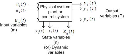
The ststae variables are usually represented as
$$ x_1(t), x_2(t),----- x_n(t) $$- n state variables
The input variable as
$$ u_1(t), u_2(t),----- u_m(t) $$- m inputs
The output variables as
$$ y_1(t), y_2(t),----- y_p(t) $$-p outputs
Fig. 2. The state variable representation of a control system
In vector matrix form
X(t)= $$\begin{bmatrix}
x_1(t)
x_2(t)
.
.
.
x_n(t)
\end{bmatrix}_{n\times1}$$;
U(t)=$$\begin{bmatrix}
u_1(t)
u_2(t)
.
.
.
u_n(t)
\end{bmatrix}_{m\times1}$$;
Y(t)=$$\begin{bmatrix}
y_1(t)
y_2(t)
.
.
.
y_p(t)
\end{bmatrix}_{p\times1}$$......................................(5)
Note: Some text books refers matrix as $$\bar{x}(t), \bar{u}(t)$$ and $$\bar{y}(t)$$.
For a given mechanical system, the state variable representation is given by two first-order differential equations, and the solution of these two equations gives the state variables x(t), v(t) of the system.
So, for a general system shown in block diagram, the state variable representation can be written as 'n' $$ 1^{st} $$ order differential equations.
$$ \frac{dx_1(t)}{dt}=\dot{x_1}(t)=f_1(x_1, x_2,........x_n, u_1, u_2,........u_m) $$ . .
$$ \frac{dx_n(t)}{dt}=\dot{x_n}(t)=f_n(x_1, x_2,........x_n, u_1, u_2,........u_m) $$..........................(6)
The integration of the above equation gives
$$ x_i(t)=x_i(t_0)+\int_{t_0}^{t}f_i(x_1, x_2,........x_n, u_1, u_2,........u_m)dt $$.............................(7)
where i=1, 2, 3,.........n
$$ [t_0, t] $$ is known as time interval.
The 'n' first order differential equations of (6) above, in matrix vector notation
$$ \dot X(t)=f(X(t)_{n\times1}, U(t)_{m\times1}) $$
Where f= $$\begin{bmatrix}
f_1(.),
f_2(.),
:
:
f_n(.)
\end{bmatrix}^T_{n\times1}$$ ......................................(8)
For time varying systems,f is depends on time 't' also.
$$ \dot X(t)=f(X(t), U(t), t) $$......................................(9)
So, the state equation
$$ \dot X(t)=f(X(t), U(t)) $$ for time invariant system.
$$ \dot X(t)=f(X(t), U(t), t) $$ for time-varying system.
Now, the state vector 'X(t)' determines a point [called state point] in n-dimensional space called 'state space'.
The curve traced out by the state point X(t) from $$ t=t_0 $$ to $$ t=t_1 $$ in the direction of increasing time is known as state trajectory.
Note: For two-dimensional cases, the state space reduces to state plane or phase plane [in nonlinearities].
In general, the output Y(t) can be expressed in terms of X(t) and U(t) as
$$Y(t)=\bar{g}(X(t), U(t))$$; Time invariant system ......................................(10)
$$Y(t)=\bar{g}(X(t), U(t), t)$$; Time-variant system......................................(11)
Note: The output equation is not a dynamic relation but a static (instantaneous) one. It is called the readout function.
The state (9) and output (10) equations constitute the state model of the system.
State model for the linear system:
Linear time-invariant system or LTI system:
The LTI system is a special case of the general equations (8) and (10)
The derivative of each state variable now becomes a linear combination of system states and inputs i.e
$$\dot{x_1}(t)=a_{11}x_1(t)+a_{12}x_2(t)+...+a_{1n}x_n(t)+b_{11}u_1(t)+...+b_{1m}u_m(t) $$
:
:
$$\dot{x_n}(t)=a_{n1}x_1(t)+a_{n2}x_2(t)+....+a_{nn}x_n(t)+b_{n1}u_1(t)+...+b_{nm}u_m(t) $$ ............................(12)
The coefficient $$a_{ij} $$ and $$ b_{ij} $$ are constants: In the matrix notation $$\begin{bmatrix}
\dot{x_1}(t)\\
\dot{x_2}(t)\\
.\\
.\\
\dot{x_n}(t)
\end{bmatrix}_{n\times1}=\begin{bmatrix}a_{11} & a_{12} & - & - & - & a_{1n}\\
a_{21} & a_{22} & - & - & - & a_{2n}\\
. & . \\
. & . \\
a_{n1} & a_{n2} & - & - & - & a_{nn}
\end{bmatrix}_{n\times n} \begin{bmatrix}
x_1(t)\\
x_2(t)\\
.\\
.\\
x_n(t)
\end{bmatrix}_{n\times1}$$+$$\begin{bmatrix}
b_{11} & b_{12} & - & - & - & b_{1m}\\
b_{21} & b_{22} & - & - & - & b_{2m}\\
. & . \\
. & . \\
b_{n1} & b_{n2} & - & - & - & b_{nm}
\end{bmatrix}_{P\times m}$$ $$\begin{bmatrix}
u_1(t)\\
u_2(t)\\
.\\
.\\
u_m(t)
\end{bmatrix}_{m\times 1}$$
i.e $$ \dot{X}(t)=AX(t)+BU(t)$$-state equation ............................(13)
$$\begin{bmatrix}
{y_1}(t)\\
{y_2}(t)\\
.\\
.\\
{y_p}(t)
\end{bmatrix}_{P\times1}=
\begin{bmatrix}
c_{11} & c_{12} & - & - & - & c_{1n}\\
c_{21} & c_{22} & - & - & - & c_{2n}\\
. & . \\
. & . \\
c_{p1} & c_{p2} & - & - & - & c_{pn}
\end{bmatrix}_{p\times n}
\begin{bmatrix}
x_1(t)\\
x_2(t)\\
.\\
.\\
x_n(t)
\end{bmatrix}_{n\times1}$$+$$\begin{bmatrix}
d_{11} & d_{12} & - & - & - & d_{1m}\\
d_{21} & d_{22} & - & - & - & d_{2m}\\
. & .\\
. & . \\
d_{p1} & d_{p2} & - & - & - & d_{pm}
\end{bmatrix}_{p\times m}\begin{bmatrix}
u_1(t)\\
u_2(t)\\
.\\
.\\
u_m(t)
\end{bmatrix}_{m\times 1}$$
i.e $$ Y(t)=C\times(t)+DU(t) $$- output equation............................(14)
where
X(t)-$$ n\times1 $$ state vector
U(t): $$ m\times1 $$ input vector
Y(t): $$ p\times1 $$ output vector
A: $$n\times n $$ system matrix
B: $$n\times m $$ input matrix
C: $$p\times n $$ output matrix
D: $$p\times m $$ Transmission matrix.
The block diagram representation of equations (13) and (14) as shown below.
Fig. 4: The block diagram representation of state model
Example:
For the previous mechanical system in above Fig.1, the state model is
$$ \frac{dx(t)}{dt}=v(t)$$
$$\frac{dv(t)}{dt}=\frac{1}{M}F(t) $$
Let us define
Here input is f(t)=u(t), output is x(t)
state variables $$x_1(t), x_2(t)$$
where $$x_1(t)$$=x(t)
and $$ x_2(t)=v(t)=\dot x(t)=\dot x_1(t) $$
$$ \dot x_1(t)=x_2(t) $$
$$ \Rightarrow \dot x_2(t)=\frac{1}{M}u(t) $$
$$ \begin{bmatrix}
\dot x_1(t)\\
\dot x_2(t)
\end{bmatrix}=\begin{bmatrix}
0 & 1 \\
0 & 0
\end{bmatrix}\begin{bmatrix}
x_1(t)\\
x_2(t)
\end{bmatrix}+\begin{bmatrix}
0\\
\frac{1}{M}
\end{bmatrix}u(t)$$
The output equation is
y(t)=x(t)=$$x_1(t)$$=[1 0]$$ \begin{bmatrix}
x_1(t)\\
x_2(t)
\end{bmatrix}$$
Note:
-
The state variables of a system are non unique.
-
The state variables need not be physical variables of the system.
-
All the models of a system will have the same characteristics
i.e The number of elements in the state vector is equal and minimum. And the number (n) is referred to as the 'order' of the system.
Note:
The state model for the linear time-varying system is of the same as defined in (1.13), except for the fact that the coefficients of the matrices A, B, C & D are not constants but are the function of time.
i.e $$ \dot X(t)=A(t)X(t)+B(t)U(t) $$
$$ \dot Y(t)=C(t)X(t)+D(t)U(t). $$
State model of the single input and single output system: [SISO-Linear system]
Since the transfer function models deal mainly with single input-single output linear time-invariant systems, the state variable model (to link) also studied by assuming m=1(input) and p=1 (output)
And the systems are classified into two categories.
1. Weekly coupling systems[SISO-classical approach]
2. Strongly coupling systems[MIMO-modern control theory/ advanced control theory]
Based on the study of every output for every input, this is referred to as interaction (or) coupling.
In the first case, the one input effects only one output, and others weekly effects, but not in the $$ 2^{nd} $$ case.
So, the MIMO systems broken-up into SISO systems for studying analysis and design. Thus the SISO system can be represented as
$$ \dot X(t)=A(t)X(t)+bu(t) $$............................(15)
$$ Y(t)=c(t)X(t)+du(t). $$............................(16)
Where
b=$$ n\times1 $$ matrix
d=$$ 1\times1 $$ a constant
c=$$ 1\times n $$ matrix
u(t)=is a scalar control variable.
The block diagram representation of (15) and (16) is as shown in below figure
Fig. 5: The block diagram representation of a state model
Note: Usually the output is not affected by inputs. So we can neglect the d and written as y(t)=CX(t)
Example: Represent system with $$ \frac{Y(s)}{U(s)}=\frac{s+3}{s+1}$$ in state model
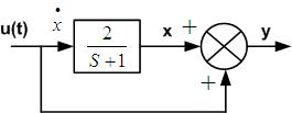
Given $$ \frac{Y(s)}{U(s)}=\frac{s+3}{s+1}=1+\frac{2}{s+1} $$
The above is represented in block diagram from as below
Fig. 6: The block diagram of given system
$$ \Rightarrow \dot x(t)+x(t)=2u(t) $$
$$ \dot x(t)=-x(t)+u(t) $$ where $$ d\neq 0 $$
-
For control system to be low pass filter, then the power of denominator is greater than $$ N_r $$
-
We get u(t) in O/P equation only when the degree of $$ D_r $$ & $$ N_r $$ are equal.
-
Hence for general control systems [low pass filter, allows useful frequencies, and rejects unuseful] does not appear in the output equation.
Non-unique property of state variables choice:
Consider the mechanical system shown in Fig. 1 where $$ x_1(t)=x(t); x_2(t)=v(t) $$ are chosen as state variables.
Now we can define the variable as
$$ z_1(t)=2x(t)+v(t) $$
$$ z_2(t)=x(t)+v(t) $$ OR $$ X_1(t)=Z_1(t)-Z_2(t) $$ $$ v(t)=2z_2(t)-z_1(t) $$
Now $$ \frac{dz_1(t)}{dt}=\dot{z_1}(t)=2\frac{dx(t)}{dt}+\frac{dv(t)}{dt} $$
$$ =2v(t)+\frac{1}{M}F(t) $$
$$ =2[2z_2(t)-z_1(t)]+\frac{1}{M}F(t) $$
$$ =-2z_1(t)+4z_2(t)+\frac{1}{M}F(t) $$
and $$ \frac{dz_2(t)}{dt}=\dot{z_2}(t)=2\frac{dx(t)}{dt}+\frac{dv(t)}{dt} $$
$$ =v(t)+\frac{1}{M}F(t) $$
$$ -z_1(t)+2z_2(t)+\frac{1}{M}F(t) $$
So, the state equation with new state variables is
$$\begin{bmatrix}
\dot z_1(t)\\
z_2(t)
\end{bmatrix}=\begin{bmatrix}
-2 & 4\\
-1 & 2
\end{bmatrix}\begin{bmatrix}
z_1(t)\\
z_2(t)
\end{bmatrix}+\begin{bmatrix}
\frac{1}{M}\\
\frac{1}{M}
\end{bmatrix}F(t)$$ ............................(17)
The output equation
$$y(t)=x(t)=z_1(t)-z_2(t)=[1 -1]
\begin{bmatrix}
z_1(t)\\
z_2(t)
\end{bmatrix}$$ ............................(18)
The above two state equations are alternative to previous one, so we conclude that choice of state variables is non-unique and state models are infinitely many will possible, among which some models defined with state variables may simple and more useful than the other choice of state models.
State Variable Representation
In state space, the choice of a state variable is arbitrary, but the possible choices are
1. Physical variables
2. Phase variables.
Physical variables state space representation:
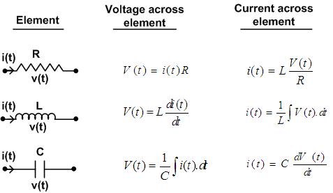
The physical variables of Electrical systems are Current and Voltage in resistance (R), inductance (L) & capacitance (C) [fundamental elements]
The basic model of the electrical system is obtained by using R, L, & C, with these we can write electrical network (or) equivalent network of the system.
By applying Kirchhoff's Current Law (KCL) at various nodes and Kirchhoff's Voltage Law(KVL) at various closed loops in the network.
The current and voltage relationships in R, L, & C.
Note:
-
The best choice of state variables in the electrical networks (or) systems is current & voltage in energy storage elements. i.e., L & C
-
The inputs to the electrical system are exciting voltage source or exciting current source.
-
The outputs in the electrical systems are voltage & current in energy dissipating element which is 'R'- Resistance.
Physical systems & state assignment:
Generally, the physical systems are,
-
Mechanical systems
-
Electrical systems
-
Liquid level systems
-
Thermal systems
Mechanical systems:
Translational:
Potential Energy =$$\frac{1}{2}mv^2$$
Kinetic Energy =$$\frac{1}{2}Ky^2$$
where v=velocity y=displacement
Ratational :
Potential Energy= $$\frac{1}{2}J\omega^2$$
Kinetic Energy = $$\frac{1}{2}K\theta^2$$
In mechanical systems y, $$\theta$$, v & $$\omega$$ are taken as state variables.
2. Electrical systems:
Energy = $$\frac{1}{2}Cv^2$$, or $$\frac{1}{2}Li^2$$
$$ i=C\frac{dv}{dt}$$; or $$ L\frac{di}{dt}=v$$
Current 'i' through the inductor & voltage 'v' across the capacitor is taken as state variables.
3. Liquid level systems:
Energy stored =$$\frac{1}{2}cP^2$$
where P=Pressure
c=Hydraullic capacity or capacitor which depends on the area of cross section and density.
$$P=\rho g h$$
where $$\rho$$- density, g- gravity, h- height of the liquid in the tank is taken as state variable.
4. Thermal systems:
Without heat carrier $$\rightarrow$$ Ex: heater
With heat carrier $$\rightarrow$$ Ex: Liquid heater
Heat Energy: $$MC\theta$$
where M=Mass
C=Specific heat capacity
$$\theta$$= Temperature.
$$`\theta'$$ is taken as a state variable.
Problem Type 1. To obtain state model from the physical system model-Physical Variable Model.
Example 1: Obtain the state space representation of the following network given in Fig. 7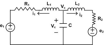
Fig. 7: Electrical Network
Solution:
Loop-1:
$$ L_1\frac{di_1}{dt}+i_1R_1+e_1-V_c=0 $$
$$ \frac{di_1}{dt}=-\frac{R_1}{L_1}i_1-\frac{e_1}{L_1}+\frac{V_c}{L_1} $$
Loop-2:
$$ L_2\frac{di_2}{dt}+i_2R_2+e_2-V_c=0 $$
$$ \frac{di_2}{dt}=-\frac{R_2}{L_2}i_2-\frac{e_2}{L_2}+\frac{V_c}{L_2} $$
KCL at $$ V_c $$:
$$ C\frac{dV_c}{dt}\neq i_1+i_2=0 $$
$$ \frac{dV_c}{dt}=-i_1-i_2 $$
State equation
$$ \begin{bmatrix}
\dot{i_1}\\
\dot{i_2}\\
\dot{v_c}
\end{bmatrix}=
\begin{bmatrix}
-\frac{R_1}{L_1} & 0 & \frac{1}{L_1} \\
0 & -\frac{R_2}{L_2} & \frac{1}{L_2}\\
-\frac{1}{C} & -\frac{1}{C} & 0
\end{bmatrix}+
\begin{bmatrix}
-\frac{1}{L_1} & 1\\
0 & \frac{1}{L_2}\\
0 & 0
\end{bmatrix}
\begin{bmatrix}
e_1\\
e_2
\end{bmatrix}$$
Let output $$ y=i_1 $$ and
Output equation is
y=$$\begin{bmatrix}1 & 0 & 0\end{bmatrix}\times \begin{bmatrix}
i_1\\
i_2\\
v_c
\end{bmatrix}+ 0 $$
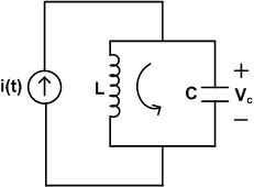
Example 2: Obtain the state space representation of the following network given in Fig. 8
Fig. 8: Electrical Network
Solution:
i(t)=$$ i_L+i_c $$
$$ i(t)=i_L+c\frac{dV_c}{dt} $$
$$ \frac{dV_c}{dt}=-\frac{-i_L}{C}+\frac{i(t)}{C} $$
$$ L\frac{di_L}{dt}-V_c=0 \Rightarrow \frac{di_L}{dt}=\frac{V_c}{L} $$
$$\begin{bmatrix}
\frac{dV_c}{dt}\\
\frac{di_L}{dt}
\end{bmatrix}=
\begin{bmatrix}
0 & \frac{-1}{c}\\
\frac{1}{L} & 0
\end{bmatrix}
\begin{bmatrix}
V_c\\
i_L
\end{bmatrix}+
\begin{bmatrix}
\frac{1}{c}\\
0
\end{bmatrix} i(t) $$
Problem Type 2: To obtain state model from Differential Equations- Phase Variable Model
Example 1: Obtain the state model of the following system represented by differential equation
$$ \frac{d^3y}{dt^3}+4\frac{d^2y}{dt^2}+8\frac{dy}{dt}+12y=10u $$
Solution:
Laplace Transformation (LT) of above equation :
$$ [s^3+4s^2+8s+12]Y(s)=10U(s) $$
$$ \frac{Y(s)}{U(s)}=\frac{10}{s^3+4s^2+8s+12}$$
Define state variables as
let $$ y=x_1 $$
$$ \frac{dy}{dt}=\dot{x_1}=x_2 $$
$$ \frac{d^2y}{dt^2}=\dot{x_2}=x_3 $$
$$ \frac{d^3y}{dt^3}=\dot{x_3} $$
and State equations can be written as
$$\dot{x_1}=x_2 $$
$$ \dot{x_2}=x_3 $$
$$ \dot{x_3}=10u-4x_3-8x_2-12x_1 $$
In the matrix form
$$\begin{bmatrix}
\dot{x_1}\\
\dot{x_2}\\
\dot{x_3}
\end{bmatrix}=
\begin{bmatrix}
0 & 1 & 0\\
0 & 0 & 1\\
-12 & -8 & -4
\end{bmatrix}
\begin{bmatrix}
x_1\\
x_2\\
x_3
\end{bmatrix}+
\begin{bmatrix}
0\\
0\\
1\\
\end{bmatrix} u(t) $$
Output y(t)=$$x_1(t)$$ and in matrix notation
y=$$\begin{bmatrix}1& 0 &0\end{bmatrix} \times \begin{bmatrix}
x_1\\
x_2\\
x_3
\end{bmatrix}+[0]u(t) $$
Example 2: Obtain state model of $$ \frac{Y(s)}{U(s)}=\frac{10(s^2+6s+12)}{s^3+2s^2+3s+9} $$
Solution:
$$\begin{bmatrix}
\dot{x_1}\\
\dot{x_2}\\
\dot{x_3}
\end{bmatrix}=
\begin{bmatrix}
0 & 1 & 0\\
0 & 0 & 1\\
-9 & -3 & -2
\end{bmatrix}
\begin{bmatrix}
x_1\\
x_2\\
x_3
\end{bmatrix}+
\begin{bmatrix}
0\\
0\\
1
\end{bmatrix} u $$
y=$$\begin{bmatrix}12 & 6 &1\end{bmatrix}$$
$$\begin{bmatrix}
x_1\\
x_2\\
x_3
\end{bmatrix}+[0]u $$
Problem Type 3: To obtain Transfer function from state model
Solution:
$$ \dot{X}(t)$$=A X(t)+B U(t)
$$Y(t)=C X(t)+D U(t)$$
Applying Laplace transform
$$s X(s)-X(0)=A X(s)+B.U(s) .........................(1)$$
$$Y(s)=C X(s)+D U(s).....................(2)$$
Transfer function is defined under initial conditions $$X(0)=0$$
From (1)
$$(sI-A)X(s)=B U(s)$$
$$ Rightarrow X(s)=(sI-A)^{-1}.B.U(s) $$ substituting in (2)
$$ Y(s)=[C(sI-A)^{-1}.B+D]U(s) $$
Transfer Function (TS) is
$$ \frac{Y(s)}{U(s)}=C(sI-A)^{-1}.B+D $$
Example 1: Find transfer function of the system with TS $$ \frac{Y(s)}{U(s)}=\frac{1}{s^4+5s^3+8s^2+6s+3} $$
reverse order with reverse sign
Solution:
$$\begin{bmatrix}
\dot{x_1}\\
\dot{x_2}\\
\dot{x_3}\\
\dot{x_4}
\end{bmatrix}$$ =$$\begin{bmatrix}
0 & 1 & 0 & 0\\
0 & 0 & 1 & 0\\
0 & 0 & 0 & 1\\
-3& -6& -8& -5
\end{bmatrix}
\begin{bmatrix}
x_1\\
x_2\\
x_3\\
x_4
\end{bmatrix}+
\begin{bmatrix}
0\\
0\\
0\\
1
\end{bmatrix} u $$
Y(t)=[1 0 0 0]$$\begin{bmatrix}
x_1\\
x_2\\
x_3\\
x_4
\end{bmatrix}+[0]u $$
Example:
Solution:
$$ \frac{d^2y}{dt^2}+\frac{dy}{dt}+9y=2\frac{du}{dt}+u $$
$$ (s^2+7s+9)Y(s)=(2s+1)U(s) $$
$$ \frac{Y(s)}{U(s)}=\frac{2s+1}{s^2+7s+9} $$
Phase Variable Method:
$$ \frac{Y(s)}{U(s)}=\frac{1}{s^2+7s+9}(2s+1) $$
$$ \Rightarrow $$ Denominator we consider for state equation
$$ \Rightarrow $$ Numerator for output equation
$$\begin{bmatrix}
\dot X_1\\
\dot X_2\\
\end{bmatrix}=\begin{bmatrix}
0&1\\
-9&-7
\end{bmatrix} \begin{bmatrix}
X_1\\
X_2
\end{bmatrix}+ \begin{bmatrix}
0\\
1
\end{bmatrix}u$$
Y=$$\begin{bmatrix}1 & 2 \end{bmatrix}$$\begin{bmatrix}
X_1\\
X_2
\end{bmatrix}+[0]u $$
Stability for State Models:
$$ \frac{Y(s)}{C(s)}=C.[SI-A]^{-1}.B+D $$
$$ =\frac{C.Adj[SI-A]}{|SI-A|}.B+D $$
$$ \frac{Y(s)}{C(s)}=\frac{C.Adj[SI-A].B+|SI-A|.D}{|SI-A|} $$
Zero's=$$ C.Adj[SI-A].B+|SI-A|.D=0 $$
Poles$$(1+G(s)H(s))=|SI-A|=0$$
Eigen values of system matrix[A]=C.L.poles
Example:
Solution:
$$ \dot X=\begin{bmatrix}
0& 1\\
-20&-9
\end{bmatrix} X+\begin{bmatrix}
0\\
1
\end{bmatrix} r $$
C=[-17 -5] X+[1]r
sI-A=$$\begin{bmatrix}
s&0\\
0&s
\end{bmatrix}-\begin{bmatrix}
0&1\\
-20&-9
\end{bmatrix}=
\begin{bmatrix}
s&-1\\
20&s+9
\end{bmatrix}$$
Adj[sI-A]=$$\begin{bmatrix}
s+9&1\\
-20&s
\end{bmatrix}$$
Adj[sI-A].B=$$\begin{bmatrix}
s+9&1\\
-20&s
\end{bmatrix}
\begin{bmatrix}
0\\
1
\end{bmatrix}=
\begin{bmatrix}
1\\
s
\end{bmatrix}$$
C.Adj[sI-A].B=[-17 -5]$$\begin{bmatrix}
1\\
s
\end{bmatrix}=[-17 -5s]$$
|(sI-A)|=s(s+9)+20
(sI-A).D=$$[s^2+9s+20][1]$$
Example:
Solution:
$$ \dot X\begin{bmatrix}
-1&0\\
0&-2
\end{bmatrix}X+\begin{bmatrix}
1\\
0
\end{bmatrix} u; $$Y=$$ \begin{bmatrix}
1\\
0
\end{bmatrix}^T $$
(sI-A)=$$\begin{bmatrix}
s&0\\
0&s
\end{bmatrix}-\begin{bmatrix}
-1&0\\
0&-2
\end{bmatrix}$$
=$$\begin{bmatrix}
s+1&0\\
0&s+2
\end{bmatrix}$$
Adj[sI-A]=$$\begin{bmatrix}
s+2&0\\
0&s+1
\end{bmatrix}$$
|(sI-A)|=(s+1)(s+2)
$$ [sI-A]^{-1}=\begin{bmatrix}
\frac{1}{s+1} & 0\\
0 & \frac{1}{s+2}
\end{bmatrix} $$
$$ [sI-A]^{-1}.B=\begin{bmatrix}
\frac{1}{s+1} & 0\\
0 & \frac{1}{s+2}
\end{bmatrix}
\begin{bmatrix}
1\\
0
\end{bmatrix}=
\begin{bmatrix}
\frac{1}{s+1}\\
0
\end{bmatrix}$$
$$ C=[sI-A]^{-1}.B\Rightarrow [1 1]
\begin{bmatrix}
\frac{1}{s+2}\\
0
\end{bmatrix} =\frac{1}{s+2}$$
shortcut: Observe 'B' and Poles then decide
EX: $$ \dot X(t)=-2\times(t)+2U(t) $$
$$ y(t)=0.5x(t) $$
L.T:
$$sX(s)=-2X(s)+2U(s)$$
$$(s+2)X(s)=2U(s)$$
$$ X(s)=\frac{2}{s+2}U(s) $$
$$ Y(s)=\frac{1}{2}X(s) $$
$$ \frac{1}{2}\frac{1}{s+2}U(s) $$
$$ \frac{Y(s)}{U(s)}=\frac{1}{s+2} $$
Problem: Diagnolization of System matrix (A).
$$ \dot X= AX+BU $$
$$Y= CX+DU$$
Let $$X=Pz$$ [Transformation matrix]
$$ P\dot z=APz+BU $$
$$Y=CPz+DU$$
$$ \dot z=[P^{-1}AP]z+[P^{-1}.B]u $$
$$Y=CPz+DU$$
P=$\begin{bmatrix}
1&1&1&-&-&-&1\\
\delta_1&\delta_2&\delta_3&-&-&-&\delta_n\\
\delta_1^2&\delta_2^2&\delta_3^2&-&-&-&\delta_n^2&\\
-&-&-&-&-&-&-\\
-&-&-&--&-&-&-\\
\end{bmatrix}$ =Vander monde matrix
$P^{-1}AP$=Diagonal matrix with diagonal elements are EIGEN VALUES
Example 5:
Diagonalise A=
$\begin{bmatrix}
0&1\\
-6&-5
\end{bmatrix}$
solution:
$ sI-A\Rightarrow
\begin{bmatrix}
s&0\\
0s
\end{bmatrix}-
\begin{bmatrix}
0&1\\
-6&-5
\end{bmatrix}=
\begin{bmatrix}
s&-1\\
6&s+5
\end{bmatrix}$
|sI-A|=0$ \Rightarrow $ s(s+5)+6=0
$ s^2+5s+6=0 \Rightarrow -2,-3 $
p=
$\begin{bmatrix}
1&1\\
-2&-3
\end{bmatrix}$
$ p^{-1}=\frac{Adj p}{|p|}=
\begin{bmatrix}
3&1\\
-2&-1
\end{bmatrix}$
Diagonal matrix$[P^{-1}AP]\Rightarrow
\begin{bmatrix}
3&1\\
-2&1
\end{bmatrix}
\begin{bmatrix}
0&1\\
-6&-5
\end{bmatrix}
\begin{bmatrix}
1&1\\
-2&-3
\end{bmatrix}$
zero's $ \Rightarrow-17-5s+s^2+9s+20=0 $
$ s^2+4s+3=0 $
zero's$ \Rightarrow -1, -3 $
Poles=|sI-A|=0
$ s^2+9s+20=0 $
Poles=-4, -5
Poles lie on LHS of s-plane.
$\therefore$ System is Stable
Example 6:
$\dot x=
\begin{bmatrix}
0&1&0\\
0&0&1\\
0.5&1&2
\end{bmatrix}x+
\begin{bmatrix}
0\\
0\\
1
\end{bmatrix}u $
u=[-0.5 -3 -5]X+U
solution:
$\dot x=
\begin{bmatrix}
0&1&0\\
0&0&1\\
0.5&1&2
\end{bmatrix}x+
\begin{bmatrix}
0\\
0\\
1
\end{bmatrix}_{3\times1}[-0.5 -3 -5]_{1\times3}+
\begin{bmatrix}
0\\
0\\
1
\end{bmatrix}V $
$ \begin{bmatrix}
0&1&0\\
0&0&1\\
0.5&1&2
\end{bmatrix}X+
\begin{bmatrix}
0&0&0\\
0&0&0\\
-0.5&-3&-5
\end{bmatrix}X +
\begin{bmatrix}
0\\
0\\
1
\end{bmatrix}V$
$\begin{bmatrix}
0&1&0\\
0&0&1\\
0&-2&-3
\end{bmatrix}X+
\begin{bmatrix}
0\\
0\\
1
\end{bmatrix}V$
Shortcut:
sum of principle diagonal elements=sum eigen values
| sI-A |=
$\begin{bmatrix}
S&1&0\\
0&S&0\\
0&0&S
\end{bmatrix}-
\begin{bmatrix}
0&1&0\\
0&0&1\\
0&-2&-3
\end{bmatrix}$
=$\begin{bmatrix}
s&-1&0\\
0&s&-1\\
0&2&s+3
\end{bmatrix}$
problem type 4:
Solution of state equation:
$\dot{x}(t)=A x(t)+B u(t)$
(a) Free response [u(t)=0]
$\dot{x}(t)=A x(t)$
\begin{equation} \label{axt}
\dot{x}(t)-A x(t)=0
\end{equation}
$x(t)==ke^{At}$
Apply L.T to eqn (axt)
$sX(s)-x(0)-A X(s)=0$
$(sI-A)x(s)=X(0)$
$X(s)=(sI-A)^{-1}x(0)$
$(sI-A)^{-1}$ called Resolvant matrix
$x(t)=\{L^{-1}(sI-A)^{-1}\}x(0)$
$x(t)=e^{-At}x(0)$
$s(t)=e^{At}=L^{-1}(sI-A)^{-1}$
State transition matrix.
(b) Forced response:
$$sX(s)-X(0)=AX(s)+BU(s)$$
$$sX(s)-AX(s)=X(0)+BU(s)$$
$$(sI-A)X(s)=X(0)+B U(s)$$
$X(s)=(sI-A)^{-1}X(0)+(sI-A)^{-1}B U(s)$
$x(t)=\{L^{-1}(sI-A)^{-1}\}x(0)+L^{-1}[((sI-A)^{-1}).B.U(s)]$
Canonical variable form:
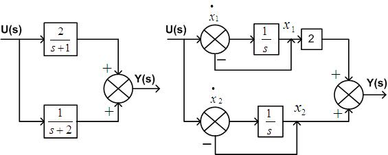
$$ \frac{Y(s)}{U(s)}=\frac{3s+5}{(s+1)(s+2)}=\frac{2}{s+1}+\frac{1}{s+2} $$
$$ Y(s)=\frac{2.U(s)}{s+1}+\frac{1.U(s)}{s+2} $$
$$ \dot x_1=-x_1+u $$
$$ \dot -2x_2=-x_1+u $$
$$ Y_1=2x_1+x_2 $$
$ \dot x_1=-x_1+u $
$ \dot -2x_2=-x_1+u $
$ Y_1=2x_1+x_2 $
$\begin{bmatrix}
\dot x_1\\
\dot x_2
\end{bmatrix}=
\begin{bmatrix}
-1&0\\
0&-2
\end{bmatrix}
\begin{bmatrix}
x_1\\
x_2
\end{bmatrix}+
\begin{bmatrix}
1\\
1
\end{bmatrix}u$
Y=[2 1]$\begin{bmatrix}
x_1\\
x_2
\end{bmatrix}$
Residues of partial factors
shortcut:
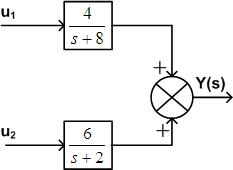
problem:
$\begin{bmatrix}
\dot x_1\\
\dot x_2
\end{bmatrix}=
\begin{bmatrix}
-8&0\\
0&-2
\end{bmatrix}
\begin{bmatrix}
x_1\\
x_2
\end{bmatrix}+
\begin{bmatrix}
1&0\\
0&1
\end{bmatrix} u$
Y=[4 6]$\begin{bmatrix}
X_1\\
x_2
\end{bmatrix}$
EX: ZIR$ \rightarrow $ free response
shortcut method:
At $t=0$
$X(t)=X(0)$
$\dot X=\begin{bmatrix}
1&0\\
1&1
\end{bmatrix}X;$ X(0)=$\begin{bmatrix}
1\\
0
\end{bmatrix}$
sI-A=$\begin{bmatrix}
s&0\\
0&s
\end{bmatrix}-
\begin{bmatrix}
1&0\\
1&1
\end{bmatrix}=
\begin{bmatrix}
s-1&0\\
-1&s-1
\end{bmatrix}$
$ [sI-A]^{-1}=\begin{bmatrix}
\frac{1}{s-1}&0\\
\frac{1}{(s-1)^2}&\frac{1}{s-1}
\end{bmatrix} $
$\begin{bmatrix}
\dot x_1\\
\dot x_2
\end{bmatrix}=
\begin{bmatrix}
-8&0\\
0&-2
\end{bmatrix}
\begin{bmatrix}
x_1\\
x_2
\end{bmatrix}+
\begin{bmatrix}
1&0\\
0&1
\end{bmatrix} u$
Y=[4 6]$\begin{bmatrix}
X_1\\
x_2
\end{bmatrix}$
EX: ZIR$ \rightarrow $ free response
shortcut method:
At $t=0$
$X(t)=X(0)$
$\dot X=\begin{bmatrix}
1&0\\
1&1
\end{bmatrix}X;$ X(0)=$\begin{bmatrix}
1\\
0
\end{bmatrix}$
$sI-A$=$\begin{bmatrix}
s&0\\
0&s
\end{bmatrix}-
\begin{bmatrix}
1&0\\
1&1
\end{bmatrix}=
\begin{bmatrix}
s-1&0\\
-1&s-1
\end{bmatrix}$
$ [sI-A]^{-1}=\begin{bmatrix}
\frac{1}{s-1}&0\\
\frac{1}{(s-1)^2}&\frac{1}{s-1}
\end{bmatrix} $
S.T.M=$s(t)=$ e^{At}$=\begin{bmatrix}
e^t&0\\
te^t&t
\end{bmatrix} $
$X(t)$=$\begin{bmatrix}
e^t&0\\
te^t&t
\end{bmatrix}
\begin{bmatrix}
1\\
0
\end{bmatrix}=
\begin{bmatrix}
e^t\\
te^t
\end{bmatrix}$
problem type 4:
Solution of State Equation
$ \dot x(t)=Ax(t)+Bu(t) $
a). Free response [u(t)=0]
$ \dot x(t)=Ax(t)$
$ \dot x(t)-Ax(t)=0$
$ x(t)=Ke^{At} $
Apply L.T to equn. 1
$sX(s)-X(0)-AX(s)=0$
$(sI-A)X(s)=X(s)$
$X(s)$=$(SI-A)^{-1}x(0)$
$(SI-A)^{-1}$= Resolvent matrix
X(t)=$ \{L ^{-1}(sI-A)^{-1}\}X(0) $
X(t)=$ e^{At}.K $
$ s(t)=e^{At}=L^{-1}(sI-A)^{-1} $
STATE TRANSITION MATRIX
(b). Forced response:
$SX(s)-X(0)=AX(s)+BU(s)$
$SX(s)-AX(0)=X(0)+BU(s)$
$(SI-A)X(s)=X(0)+BU(s)$
$ X(s)=(SI-A)^{-1}x(0)+(SI-A)^{-1}BU(s) $
$ X(t)=\{L^{-1}(SI-A)^{-1}\}X(0)+L[(si-a)^{-1}.B.U(s)] $
Q1 :
What are the advantages of state space analysis?
Ans:
Q2 :
Define state, state variable, state vector, state space and state equations?
Ans:
Q3 :
What are the limitations of transfer function analysis?
Ans:
Q4 :
Derive from fundamentals the state equation of nth order system?
Ans:
Q5 :
Define state diagram and what are the basic elements required to construct a state diagram?
Ans:
Q6 :
Obtain the state space representation of an nth order time-invariant system with ‘r’ number of forcing functions:
Ans:
Q7 :
Define phase variable form of a state model. What are the advantages and disadvantages of a phase variable model of a state space system? What is bush form or companion form of a state model?
Ans:
Q8 :
Write the controllable canonical form of state model an nth order time-invariant system. What are the advantages and disadvantages of a canonical form of state model?
Ans:
Q9 :
Write the diagonal canonical form of state model an nth order time-invariant system?
Ans:


0 Doubts's